Biotic interactions and jSDM – report from a workshop at the Ecology Across Borders conference in Ghent, Dez 2017

This guest post by Carsten F. Dormann, with inputs from Casper Kraan and the panel (see below) summarises the results from the short workshop “Biotic interactions and joint species distribution models” at the Ecology Across Borders BES/GfÖ/NEVECOL/EEF-meeting 2017 in Ghent, Belgium. The purpose of this event was to exchange thoughts and questions about joint Species Distribution Models (jSDMs) and their ecological interpretation, in particular as indicators of biotic interactions.

Update Aug 2018: a recent publication by some of the panel participants discusses many similar and related points Dormann, Carsten F., et al. (2018) Biotic interactions in species distribution modelling: 10 questions to guide interpretation and avoid false conclusions. Global Ecology and Biogeography, in press.

1 The Panel

The workshop was organised and moderated by Carsten Dormann and Casper Kraan (who regrettably was ill and could not attend). A panel of five people using/developing jSDMs answered questions (or comment on points of views) expressed by the workshop participants (“audience”): Heidi Mod (Uni Lausanne, CH), Jörn Pagel (Uni Hohenheim, D), Melinda de Jonge (Radboud Uni, NL), Florian Hartig (Uni Regensburg, D) and Nick Golding (Uni Melbourne, AUS).

2 Introduction (CFD & CK)

In the workshop, we implicitly expected some familiarity with jSDMs, either passively (as readers of some of those recent papers), or actively (as users of the various available softwares). For novices, who want to get an idea of what jSDMs are, how they may be constructed and applied, we provide here a short introduction that was not part of the workshop.

2.1 Separating biotic interactions and environment

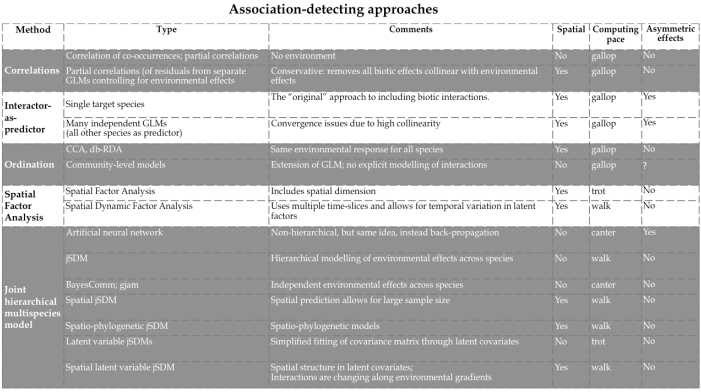
Attempts to fit/plot/understand associations among species is, of course, much older than jSDMs. For example, Braun-Blanquet (1964) called consistently occurring plant communities “associations”, and vegetation scientists have used ordination to depict such associations. In this wider sense, a rich literature of methods exists to identify associations among species (Fig. 1).

Figure 1. Approaches to detect associations among species, and some of their characteristics. From Dormann et al., in revision. See also Nieto-Lugilde et al. (2017).

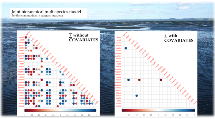
If we want to interpret species co-occurrences as positive/negative associations, it is crucial to separate the species-species signal from environmental effects on occurrence/abundance, instead of analysing “raw” co-occurrence data directly, e.g. through correlation analysis (Harris 2016). Figure 2 shows, on the left, a correlation matrix for some dozen soft-sediment marine organisms in New Zealand seagrass meadows resulting from a jSDM, and, on the right, the same correlations based on per-species residuals after accounting for environmental preferences in a jSDM. Clearly, most associations in the raw data can easily be explained by similar environmental preferences (“niches”).

Figure 2. Correlations in raw abundance data (left) and in model residuals, after removing the influence of environment in driving occurrences (right). Data and analyses by Casper Kraan, unpublished.

The idea of jSDMs is therefore to simultaneously estimate the environmental niches and species associations, where associations (“interactions”) mean residual covariation in species occurrences, after accounting for environmental effects. A good introductory review to the field is provided by Warton et al. (2015). The more recent review by Ovaskainen et al. (2017) is (even) more technical. Both share the same fundamental outlook, but emphasise different details differently. Historically, Latimer et al. (2009) were probably the first to use the “modern” form of jSDMs (i.e. linking individual regressions through their residuals), but similar approaches soon followed from other groups. Pollock et al. (2014) were the first to use the term “joint SDMs”.

2.2 Technical definitions

Technically, there are two ways in which independent SDMs can be “joined”. The first is linking their parameters, which leads to so-called multispecies models, and the second is estimating residual (after environment) species covariances, which leads to “real” jSDMs.

• Multispecies models: The idea here is using data on multiple species simultaneously for better parameter estimation. (“joint estimation”), e.g. mixed-effect models with species as random effect (see Ovaskainen & Soininen 2011, Ovaskainen et al. 2017). In a somewhat uncommon formulation, we could write that as a set of single regressions connected through hyperparameters on their parameter estimates (i.e., the random effect):
  
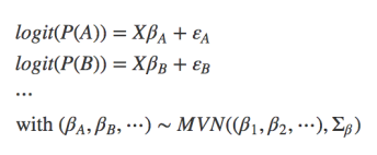
• Joint species distribution models: unlike multi-species models, which use the multiple species only to inform each other on their parameter values, a “real” jSDM looks at species associations. It can thus be defined as  “A parametric statistical model for the abundance of multiple taxa (usually species), accounting for correlation between taxa as well as response to predictor variables” (from Warton et al. 2015). In a simplified notation we could write this as:

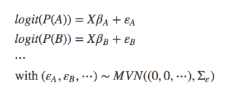
For example, BayesComm fits this (type of) jSDM, while Pollock et al. (2014) combine both parts and have both parameters and errors drawn from a multivariate normal distribution. It should also be noted that the multivariate normal distribution MNV in the formulae is the traditional choice, but this assumption could of course be relaxed to include other distributions as well.

2.3 Biotic interactions interpretation

Most discussions about jSDMs center about the association matrix, which some interpret (with qualifying statements) as hinting towards biotic interactions. This is an ecological interpretation of a so far purely statistical matrix that describes species-species associations after accounting for environmental effects.

Note that most jSDM-papers are very cautiously worded and refer to the correlations of the residuals as “associations”, rather than interactions. Indeed, Harris (2016) showed for simulated interacting communities that the compared approaches (except his mistnet approach) may easily detect spurious associations and hence would incorrectly infer biotic interactions. This conclusion seems to be corroborated by simulations of Laura Pollock, as presented the day after our workshop at the meeting, which showed that strong competitive interactions are reliably detected, but errors are high for weak or facilitative interactions.

2.4 Software

While the first approaches to jSDMs were coded in JAGS or even C, there is currently a wider selection of R-packages that can be used for this purpose. Some promising approaches are

• hmsc (https://www.helsinki.fi/en/researchgroups/metapopulation-research-centre/hmsc); this package is more advanced in its matlab version!
• boral (https://cran.r-project.org/package=boral)
• gjam (https://cran.r-project.org/package=gjam)
• Further packages:
  • spBayes (https://cran.r-project.org/package=spBayes)
  • BayesComm (https://cran.r-project.org/package=BayesComm)
  • rosalia (https://github.com/davharris/rosalia)
  • mistnet (https://github.com/davharris/mistnet)

3 Notes from the panel discussion

The following questions were collected from the audience, and then passed on to the panel. Panel responses are given in italics. Due to the shortness of time, and complexity of the topic, we could only address a few questions. Questions that were not addressed during the discussion are still listed here, but stand unanswered. Feel free to address them in the comment section. (Many thanks to Florian Hartig for his dual role of taking notes and addressing questions!)

3.1 What are the goals/possible applications of jSDMs?

• Do we have examples where jSDMs have contributed new knowledge?
  • Currently, jSDMs have generated new interpretations of the data, but also due to the difficulties of interpretation (see below), they have probably not (yet) created fundamentally new knowledge in ecology. In the future, jSDMs may eventually be used mainly as a hypothesis-generator / pattern synthesizer, possibly to be followed up by more direct / experimental investigations of detected interactions / species associations.
• When can we clearly interpret co-occurrence as a signal of ecological interactions?
  • Rarely, see also discussion below. jSDMs highlight co-occurrence patterns that deviate from environment-only expectations. There are several explanations for such a pattern, of which a true biotic interaction is only one possibility. Moreover, a positive signal at a particular scale (e.g. 10km grid) does not necessarily mean that a biotic interaction is positive / facilitative. Also with a predator-prey interaction, one might find both species more likely close to each other than expected from pure environment. 

3.2 Technical questions

• How to do model selection with jSDMs?
  • Standard AIC etc. in principle possible, but the usual problems with counting df in mixed models and poorly supported by most packages. Also, runtimes are typically prohibitive to dredge jSDMs.
  • In Bayesian approaches, regularisation priors may be a good alternative to model selection.
• Can we account for spatial and temporal autocorrelation in jSDMs?
  • For spatially structured associations see Ovaskainen et al. (2016); for spatio-temporal jSDMs see Schliep et al. (2017). Also Thorson et al. (2016; Global Ecology & Biogeography 25, 1144-1158)
• What are the benefits for prediction, and can jSDMs be extrapolated?
  • Prediction may benefit from jSDMs, compared to multispecies models, but it depends on the context, e.g. on how important BIs are. Also, it must be noted that the interaction part increases model complexity and thus may increase predictive errors if the data is not sufficient to constrain these additional degrees of freedom (bias-variance trade-off)
  • Whether predictions are improved also depends on what we mean by predictions and extrapolation. There are at least three types of jSDM-based predictions: (1) conditional, i.e. providing abundances/occurrence information for all but the target species; (2) unconditional, i.e. estimating abundances/occurrences from XX alone, for all species; and (3) marginal, by integrating over all non-target species.
  • As usual, we can test predictive power and estimate predictive errors by using process-based models as references (truth), or by cross-validation if sufficiently large datasets are available.

3.3 What are the assumptions, and what are the statistical properties of these estimators?

• Statistical: are confidence intervals reliable?
  • As always in statistics – yes, when the model assumptions are met.
• Structural assumptions/confounders, how can we safeguard against missing predictors, could BIs confound environmental effects?
  • Associations are assumed to be constant, i.e. independent of the environment (but see Tikhonov et al. 2017 for a relaxation of this assumption).
  • Very difficult to safeguard against missing environmental, which are in principle always an alternative explanation for signals in the association matrix.
• How broad taxonomically and functionally/trophically should a jSDM be?
• What about asymmetric/trophic interactions? (Note: Current jSDMs fit a symmetric association matrix; thus, the effect of A on B is the same as B on A. This is rarely ecologically plausible. For an exception, see packages mistnet, referenced above and Schliep et al. 2017.)
  • Complicated. Technically, it could certainly be done, and has been done in special cases (e.g. Schliep et al 2017 GEB), but it might be computationally very costly. As argued earlier, it is anyway difficult to directly interpret association patterns between species as measures of ecological interaction strength or direction. It is therefore questionable if it is useful to invest excessive amount of energy in making these “non-interactions” ecologically realistic.

3.4 Data properties

• Detection probability, possibly variable across species, possibly interacting with other factors (also biotic).
• How to deal with very rare or very common species?
  • Could increase uncertainty, but also improve fit. In doubt, keep in the analysis.
• Are occurrence data suitable at all for inferring BIs?
  • These are ecological questions, irrespective of jSDM. Is it sensible to interpret BI at this spatial/temporal scale? Data are often not points in space/time, but aggregates over years and hundreds of square kilometers. Remember that interactions are between individuals, not species, i.e. at very small scales.
  • Is the environmental data quality high enough and does it contain important predictors?
  • Is an interaction a priori sensible, e.g. expected from experimental evidence of these species?
• Can biotic interactions drive range margins?
  • Presumably yes (Wisz et al. 2013), possibly Louthan, 2015.
• Data problems: are species maps/records uncorrelated? For example, if plant distribution data originate from vegetation releves, we actually have point-co-occurrence data. After turning them into (single-species) range maps, this information is lost, and co-occurrences in the original data may disappear after range mapping.
  • Indeed, this points to a problem in data handling. Detection probabilities may not be independent: if I expect a species in a certain vegetation, I will be on the look-out for it, thereby biasing detection probabilities and invalidating the independence among species (see Beissinger et al. 2016, Warton et al. 2016).
• How to accommodate different spatial scales of species/BIs? For example, a lynx will interact at much larger spatial extents than its prey.
• Combining data from different sources/scales?

3.5 Metacommunity analysis with jSDMs

• How to include traits and phylogeny? For an example see Abrego et al. (2017).
  • On environmental predictors (as random slope across species, e.g. by making the effect of temperature being dependent on the body size of the species)
  • As a strategy to test the plausibility of biotic interaction-interpretation.
  • Post-hoc, after the actual jSDM analysis (see talk by Jörn Pagel on the day after the workshop)
  • Possibly as a constraint on covariance-matrix.

4 Conclusions

From the comments we received on this mini-workshop, both panel and audience enjoyed the exchange of thoughts and ideas. Also, realising that many people seem to all struggle with similar issues was deemed to be very helpful.

JSDMs are a young and rapidly moving field, and both audience and panel felt that jSDMs offer many promises for ecology, but that also many challenges in application and interpretation remain. Moreover, computing times can be prohibitive for large data sets with many species. For unlimited data, we would expect jSDMs to reduce prediction errors and therefore benefit science and conservation applications, but when this approach’s benefits actually starts to outweigh its costs (increased model flexibility) requires further investigations. Interpreting associations in jSDMs as biotic interactions is risky, as it requires eliminating all other drives of co-occurrence. Ideally, jSDM results should therefore more often followed up by traditional, causal approaches such as manipulative experiments.

5 References

Abrego, N., Norberg, A., & Ovaskainen, O. (2017). Measuring and predicting the influence of traits on the assembly processes of wood-inhabiting fungi. Journal of Ecology, 105(4), 1070–1081. doi:10.1111/1365-2745.12722

Beissinger, S. R., Iknayan, K. J., Guillera-Arroita, G., Zipkin, E. F., Dorazio, R. M., Royle, J. A., & Kéry, M. (2016). Incorporating Imperfect Detection into Joint Models of Communities: A response to Warton et al. Trends in Ecology & Evolution, 31(10), 736–737. doi:10.1016/j.tree.2016.07.009

Braun-Blanquet, J., 1964. Pflanzensoziologie. Springer, Berlin, New York, 865 pp.

Harris, D.J. (2016) Inferring species interactions from co-occurrence data with Markov networks. Ecology, 97, 3308–3314.

Latimer, A.M., Banerjee, S., Sang, H., Mosher, E.S. & Silander, J.A. (2009) Hierarchical models facilitate spatial analysis of large data sets: a case study on invasive plant species in the northeastern United States. Ecology Letters, 12, 144–54.

Nieto-Lugilde, Diego, Kaitlin C. Maguire, Jessica L. Blois, John W. Williams, and Matthew C. Fitzpatrick. (2017) Multiresponse algorithms for community-level modelling: Review of theory, applications, and comparison to species distribution models. Methods in Ecology and Evolution. https://doi.org/10.1111/2041-210X.12936.

Ovaskainen, O. & Soininen, J. (2011) Making more out of sparse data: hierarchical modeling of species communities. Ecology, 92, 289–295.

Ovaskainen, O., Roy, D.B., Fox, R. & Anderson, B.J. (2016) Uncovering hidden spatial structure in species communities with spatially explicit joint species distribution models. Methods in Ecology and Evolution, 7, 428–436.

Ovaskainen, O., Gleb Tikhonov, Norberg, A., Blanchet, F.G., Duan, L., Dunson, D., Roslin, T. & Abrego, N. (2017) How to make more out of community data? A conceptual framework and its implementation as models and software. Ecology Letters, 20, 561–576.

Pollock, L.J., Tingley, R., Morris, W.K., Golding, N., O’Hara, R.B., Parris, K.M., Vesk, P. a. & McCarthy, M. a. (2014) Understanding co-occurrence by modelling species simultaneously with a Joint Species Distribution Model (JSDM). Methods in Ecology and Evolution, 5, 397–406.

Schliep, E.M., Lany, N.K., Zarnetske, P.L., Schaeffer, R.N., Orians, C.M., Orwig, D.A. & Preisser, E.L. (2017) Joint species distribution modelling for spatio-temporal occurrence and ordinal abundance data. Global Ecology and Biogeography, 27, 142–155.

Tikhonov, G., Abrego, N., Dunson, D., & Ovaskainen, O. (2017). Using joint species distribution models for evaluating how species-to-species associations depend on the environmental context. Methods in Ecology and Evolution, 8, 443–452. doi:10.1111/2041-210X.12723

Warton, D.I., Blanchet, F.G., Hara, R.B.O., Ovaskainen, O., Taskinen, S., Walker, S.C. & Hui, F.K.C. (2015) So many variables: joint modeling in community ecology. Trends in Ecology and Evolution, 30, 766–779.

Warton, D. I., Blanchet, F. G., O’Hara, R., Ovaskainen, O., Taskinen, S., Walker, S. C., & Hui, F. K. C. (2016). Extending Joint Models in Community Ecology: A Response to Beissinger et al. Trends in Ecology & Evolution, 31(10), 737–738. doi:10.1016/j.tree.2016.07.007

Wisz, M. S., Pottier, J., Kissling, W. D., Pellissier, L., Lenoir, J., Damgaard, C. F., … Svenning, J.-C. (2013). The role of biotic interactions in shaping distributions and realised assemblages of species: implications for species distribution modelling. Biological Reviews, 88, 15–30.